The last step of data analysis can be generally described as using tools to convert sequencing data into knowledge and setting it into the biological context. In this Chapter, we will focus on the most common tertiary data analysis types. Before entering tertiary analysis, it is advisable to evaluate the results of the previous steps by a set of additional checks. This way, the researcher can ensure that the data that is used as input for the final analysis steps has passed all quality control standards.

1. Quality Control Before Entering Tertiary Data Analysis
Quality controlling the results of secondary analysis data ensures that the subsequent tertiary analysis steps are conducted with high quality data and scientifically sound conclusions can be drawn from the final output. Quality control at this step is centered on verifying that the distribution of reads matches the a priori expectation and that the quantification process will provide an accurate read-out of the library input.
Alignment Rates and Read Distribution
Once the data has been aligned to a reference genome, the aligner will output basic summary statistics. These statistics usually include the percentage of reads mapped to the reference genome. For an ideal RNA-Seq library, this metric should be greater than or equal to 90 %. While alignment rates close to 70 % may still be acceptable depending on the quality of the RNA input and the reference genome used, lower alignment rates may indicate serious issues with the data set.
Using mapping rates as QC parameter is only possible when working with organisms which are well-annotated. For non-model organisms, genome assemblies and annotations are often poor and / or incomplete. In this case, low mapping rates are to be expected and are mostly caused by the reference rather than the quality of the data set.
One explanation for low mapping rates observed for well-annotated model organisms is that most reads are too short to be properly mapped to the genome. This situation can arise when highly degraded RNA is used as input, the libraries or sequencing run are poor in quality, or when the reads have been trimmed too short in length. Another potential explanation for poor mapping quality is contamination of input material with foreign RNA. Construction of the first tardigrade genome assembly is a classic and well-cited example of how contamination can negatively influence NGS library composition and lead to false conclusions1, 2. Bacterial contamination in tardigrade cultures led to an overestimation in the amount of horizontal gene transfer that occurred in this genome.
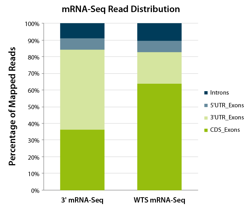
Figure 1 | Mapping class attribution for reads generated using 3’ mRNA-Seq or Whole Transcriptome mRNA Sequencing (WTS). Reads generated by 3’ mRNA-Seq are located towards the 3’ UTR of transcripts, as represented by the majority of mapped reads. In contrast, reads obtained for mRNA WTS-libraries are distributed evenly across the complete transcripts. Therefore, reads mapping to coding sequences should represent the majority of mapped reads and the fraction of reads mapping to 3’ UTRs is lower than for 3’-Seq.
When low mapping rates are observed, it may be useful to simply BLAST a portion of the unmapped reads to uncover their biological origin. However, when mapping percentages do not indicate any obvious problems, it is useful to visualize read distribution across different genomic features.
For example, RSeQC3 can be used to determine the percentage of reads which map to the CDS, 5’, and 3’ UTRs or the intronic or intergenic space. Another software with similar functionality is Picard tools.
Read distribution is an important metric which enables the user to gauge if the library contains expected read fragments. For 3’ mRNA-seq library preps such as QuantSeq, most reads should be concentrated at the 3’ UTR. In contrast, for whole transcriptome sequencing (WTS) library preps most reads typically map across the complete transcript body (Fig. 1). A concentration of reads towards the 3’ UTR would indicate degradation of the RNA sample prior to library generation. The distribution of reads over the whole exonic space or the coding sequence depends on whether upstream rRNA depletion or poly(A) selection was performed, which also has implications on the percentages of intronic and intergenic reads.
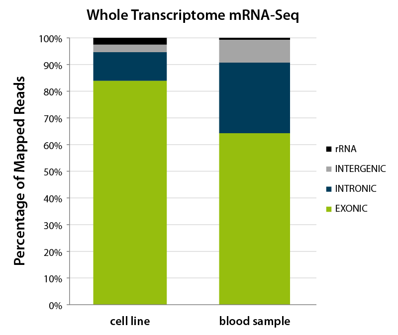
Figure 2 | Feature distribution of mapped reads from Whole Transcriptome mRNA-Seq for different sample types. The majority of reads generated from both samples type, using RNA from cell lines and from blood samples, map to exonic sequences. However, the overall distribution of reads classified as exogenic, intronic, and intergenic is changed depending on the sample type.
For example, data generated from poly(A)-selected RNA typically reflects mature mRNAs with a lower intronic and intergenic read fraction. Due to the possibility to capture pre-mature mRNA, intron-inclusion events, and the quality of the annotation itself, a certain level of intronic and intergenic reads is to be expected, whereby the intronic read percentage should be higher than the intergenic read percentage. For data generated from rRNA-depleted samples more intronic and intergenic reads are expected as this method also captures transcripts occupying this space, e.g., long (intergenic) non-coding RNAs (lncRNAs and lincRNAs). Further, commonly observed read distribution is also influenced by the sample itself. For example, RNA-Seq libraries generated from blood samples naturally show a higher distribution of reads over the intronic and intergenic space4 (Fig. 2).
A high percentage of intronic or intergenic mapping reads for samples types that routinely show lower values can indicate genomic DNA contamination (most common for WTS data, see also Chapter 5 – DNase: To Treat or Not to Treat). Further, for data obtained from 3’ -Seq libraries, such statistics can hint to mis-hybridization where oligo(dT) primers are re-directed from the poly(A) tails of mRNAs and prime to A-rich sequences present in rRNA.
Ribosomal RNA as Indicator for Library Complexity
Another important metric to examine is the percentage of ribosomal RNA (rRNA) mapping reads. While total RNA is composed of 80-98 % rRNA, quality mRNA-Seq libraries typically contain no more than single digit percentages of rRNA mapping reads.
For example, 3’ mRNA-Seq libraries, such as QuantSeq libraries, typically contain ~3-5 % rRNA mapping reads as mitochondrial rRNA transcripts contain poly(A) tails and will be captured by oligo(dT) priming together with polyadenylated mRNAs. In contrast, rRNA depleted WTS libraries, such as CORALL libraries after depletion with RiboCop, typically contain <1 % rRNA mapping reads. The content of reads derived from rRNA observed in sequencing experiments is largely dependent on the sample itself, the RNA quality and quantity, enrichment, and library preparation method. This metric should always be interpreted in relation to expected and typically observed results.
Libraries with a significantly higher fraction of rRNA are usually indicative of low complexity. This can be caused by using low amounts of RNA, or very low-quality input material which usually results in libraires with few detected genes (see Chapter 4 – RNA Extraction and Quality Control). If the genome annotation contains rRNA (some do not), the percentage of rRNA can be calculated from the output of the chosen quantifier. Ribosomal RNA percentage can also be calculated by mapping reads separately to rRNA-only sequences, which can be more accurate when using poor genome assemblies or incomplete annotations. For example, this can be done by mapping the reads to an rRNA-only database such as silva5 that contains sequences of many different organisms. As rRNA is generally highly conserved this approach can help in these cases to estimate the rRNA content.
Spike-in Controls to Assess Quantification Accuracy and Transcript Coverage
Until now, the Lexicon section on data analysis has primarily focused on read distribution across the genome and how these summary statistics can be utilized as qualitative control. While these statistics provide an adequate overview of the library content and composition, it does not tell the experimenter how accurate the quantification is. If controls such as ERCC6 spike-ins or Lexogen’s Spike-In RNA Variants (SIRVs) are added during library preparation, the researcher can use these as a ground-truth dataset to benchmark quantification performance and detection limits. Further, spike-in controls can be used to fine-tune the entire workflow including data analysis tools and parameters to deliver highly accurate results for the respective research question.
The addition of artificial spike-ins at a low read percentage does not only allow to analyze and compare data sets generated over time and across sites, it also offers the possibility to analyze a small percentage of data for a fast, initial quality control. The spike-in controls are thereby used as a proxy to assess the quality of the library generation and sequencing workflow. Should the sample show unexpected results for any of the parameters outlined above, the artificial controls can help to pinpoint the cause for the observed discrepancies. Internal controls can indicate if there was a sample-related problem, cross-contamination, or difficulties during library generation and sequencing.
2. Tertiary Data Analysis
The tertiary analysis steps depend heavily on the individual research question that was defined at the beginning of the experiment. Therefore, this part of the analysis is the most flexible during the entire project. In the upcoming section, we will therefore focus on some of the commonly used analyses, namely differential expression and functional enrichment analysis. To ensure the success of your project by generating the data you need to answer your specific research question, it is best to consult a bioinformatician prior to starting the experiment (our Chapter 3 on experimental and data analysis planning has you covered and outlines critical considerations for planning your sequencing experiment).
Differentially Gene Expression Analysis
Differential gene expression testing is one of the most common tertiary analysis methods utilized for RNA-Seq. Differential gene expression analysis is used to discover significant quantitative gene expression changes under varied biological conditions (Fig. 3 and Fig. 4).
Practical examples for differential expression studies include mapping the transcriptome changes between a wild-type and mutant, or expression changes caused by treatment with a specific stimulus or chemical compound, responses to infection, during the course of disease progression or following cell and tissue development.
Two popular tools for differential expression analysis are DESeq27 and edgeR8, both of which operate under the null hypothesis that most genes are not differentially expressed.
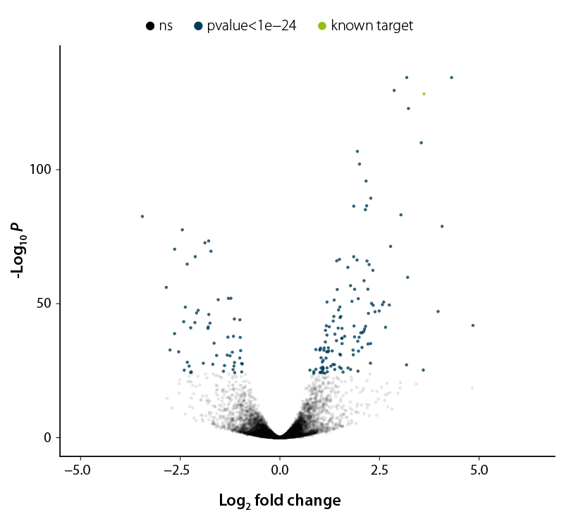
Figure 3 | Volcano Plot to distinguish significant from non-significant changes. Plotting is done based on p-values as measure of significance. Data points with low p-values correspond to highly significant changes and are plotted towards the top. Significant changes are highlighted in blue, known targets in green, and unaffected data points are shown in black. The logarithm of the fold change between the two conditions is shown on the x-axis.
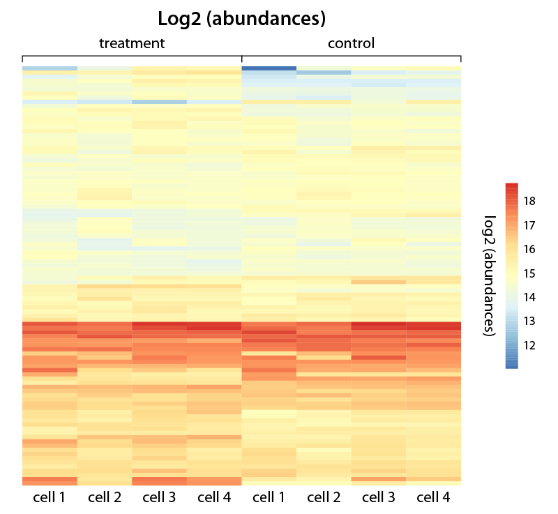
Figure 4 | Heatmap visualizing gene expression changes for various cells under two different conditions. The heat map represents color-coded expression levels of differentially expressed genes, changes in expression level are shown as log2-fold abundances.
The p-values obtained using these tools indicate the probability of a gene not being differentially regulated. Thus, a small p-value leads to a rejection of the null hypothesis and indicates significant differences in gene expression. Both DESeq2 and edgeR statistical models have been designed to work best with raw read counts6, 7. Gene length normalization is unnecessary as testing for each gene is performed separately and therefore stays constant. As raw read counts do not account for effects such as varied sequencing depths, read counts are normalized in a slightly different manner depending on the tool. For instance, DESeq2 normalizes read counts by multiplying all counts for each sample with a so called “size factor”. In concordance with the null hypothesis, these size factors are calculated with the objective to minimize the total variance across each gene for all samples. DESeq2 then estimates the dispersion for each gene (a measure of how much a sample fluctuates around a mean value) followed by a statistical test (for a detailed explanation, we recommend the resources on bioconductor.org, for example The theory behind DESeq 2).
Variations in sequencing depth can be kept low by adjusting the libraries in a lane pool according to their molarity and size distribution prior to sequencing. Equimolar pooling of each individual library enables to sequence each sample with equal read depth during the sequencing run. Even though normalizations can correct variations in read depth, reliable high-quality results are obtained when the variations are already small to begin with. Larger variations can lead to more noise and changes in expression can be harder to detect, especially when the change is rather moderate.
Tools such as DESeq2 and edgeR are also capable of performing tests for classical pairwise comparisons (e.g., control vs. treatment) and more complex scenarios such as time series or effects of a treatment on different genotypes. These complex setups are tested with a likelihood ratio test (to learn more about how these tests are performed, we recommend the resources on Bioconductor.org, for example: likelihood ratio test).
Functional Enrichment Analysis
After differential gene expression analysis has been performed, researchers often desire to gain insight into the cellular functions and molecular processes affected. One way to address this challenge is to annotate genes with metadata which describe their function. This can be achieved by analyzing information on gene-phenotype relationships, associated gene pathways, enzymatic classification of gene products, or organelle function. Once genes have been annotated with this meta data, one can crosscheck if genes of a specific pathway are enriched in the differentially regulated genes derived from the RNA seq analysis (Fig. 5). The Gene Ontology (GO) Consortium provides an excellent resource of metadata in the form of standardized terms, intended to represent current scientific knowledge of the functions of genes. GO term annotation and enrichment analysis can be performed online on the Consortiums webpage, or with standalone tools like clusterProfiler9. Both options take two lists of gene IDs as input: a background list (non-differentially regulated genes) and a list to test (differentially regulated genes). The standalone tool clusterProfiler, also allows users to incorporate other resources such as KEGG, Reactome, WikiPathways or the molecular signatures database.
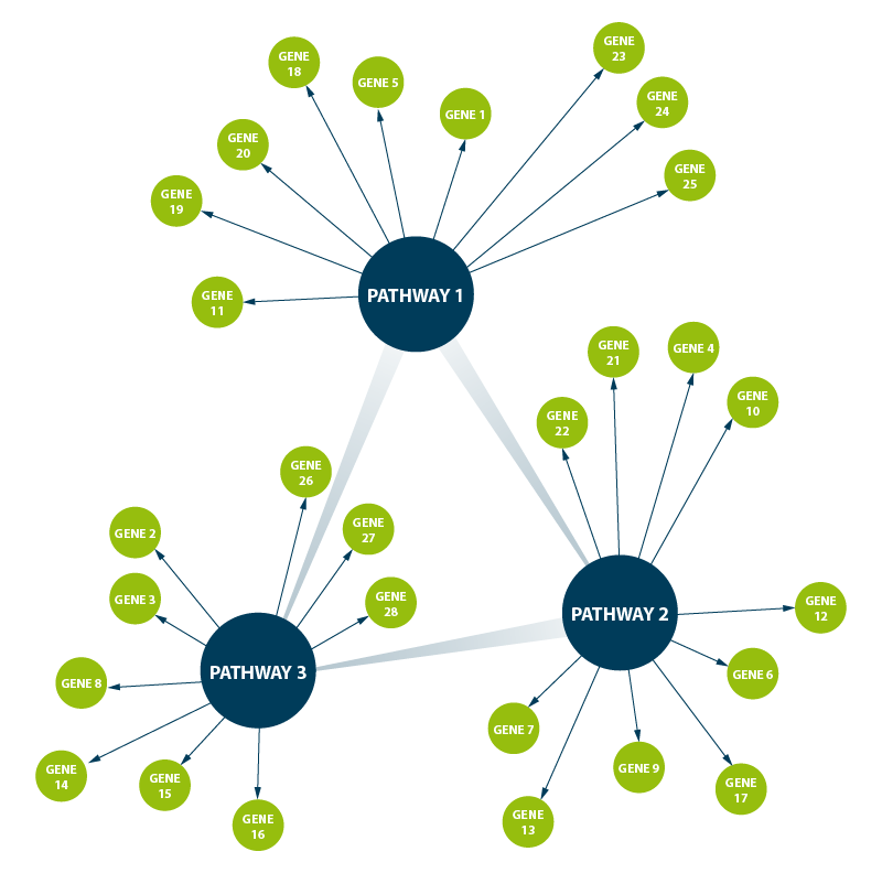
Figure 5 | Pathway analysis identifies key genes in known pathways which are altered in relation to specific conditions tested in the experiment. Genes can be up- or down-regulated leading to activated or deactivated pathways. Known interactions between pathways can help decipher signaling or regulatory cascades that are affected under the tested condition(s) and regulatory networks can be built towards the understanding of physiological changes caused by the perturbation that was tested.
3. Quality control
Using Sample-to-sample Correlation and Principal Component Analysis to QC Differential Gene Expression
As precision and accuracy of statistical testing is influenced by the reproducibly and variation within the experiment, it is useful to assess the overall similarity between samples when performing differential gene expression testing. Additionally, one should explore if the observed variation is indeed predominantly caused by the experimental conditions or influenced by other technical or biological aspects (e.g., the day of RNA isolation, operator, age, or sex of the organism etc.) This can be investigated by examining sample-to-sample correlations and by performing a principal component analysis (PCA, Fig. 6).
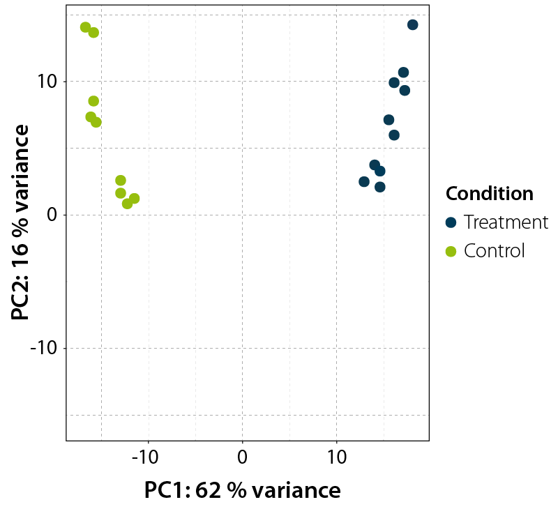
Figure 6 | Principal Component Analysis of treated and untreated control samples. RNA-Seq libraries were produced from two different conditions. Differential expression values were then evaluated in a Principal Component Analysis (PCA). The Principal Component 1 (PC1) on the x-axis clearly separates both conditions, explaining 62 % of the variability seen in the treated vs. untreated control samples clearly separating the two conditions. Replicates from both conditions cluster with less variance in Principle Component 2 (PC2).
Besides differential gene expression statistics, analysis software such as DESeq2 can also produce normalized and linearized expression data. This output can be used to calculate correlation coefficients between samples. Plotting these values in the form of a clustered heatmap is a quick and visually intuitive way to assess reproducibly between replicates and check for extreme outliners. On the other hand, PCA is a transformation technique which aims to reduce the dimensionality of data while retaining maximal variation in the data set. Gene expression data is highly dimensional, as each sample consists of several thousand data points. During PCA analysis, the information contained in these dimensions is transformed into separate uncorrelated vectors (i.e., principal components). Principle components are ordered in a way in which the first few retain most of the variation present in the original dimensions. Therefore, plotting the two principal components allow the user to obtain a summary of the variation present in the experiment (See here for a more detailed and visual explanation). In this plot (Fig. 6), one can investigate if the assigned samples groups stratify according to the experimental setup (control vs. treatment) or based on other properties (RNA isolation day, age, sex etc.). When sample groups stratify in relation to the other properties listed above, the differentially expressed genes are most likely causally related to them and not the experimental setup. The DESeq2 manual has an excellent tutorial that describes these quality control steps in practice.
Using Spike-in Controls to Validate Sample-to-sample Fold-change
Spike-in controls, such as the ERCCs can be obtained as different mixes. These mixes contain the same spike-ins but at varied concentrations and are helpful when spiked into different sample types (e.g., control vs. treatment). When these samples are then compared during differential gene expression analysis, they can be utilized to quality control fold-change estimates. Similarly, Lexogen’s SIRVs, which are available in equimolar or non-equimolar concentrations, can also be used to estimate sample-to-sample fold-changes when spiked in at comparable percentages. In addition, SIRVs contain various synthetic isoforms and thus simulate the full transcriptomic complexity. This feature makes them very useful to test RNA-Seq and data analysis workflows especially for evaluations on transcript level.
4. Tying it all together
Combining the aforementioned analysis steps into a single automated workflow is referred to as a “pipeline”. In the past, bioinformaticians mainly wrote pipelines tailored to their specific systems and needs. This was most commonly done using the UNIX shell programming language, bash. However, as the field of bioinformatics has rapidly matured, the demand for reproducible and sharable data analysis workflows has greatly increased. This demand has led to the development of sophisticated pipeline managers such as Snakemake or Nextflow, which enable greater reproducibility and ease of sharing.
NextFlow is also utilized by the nf-core project10 which is a community effort to build curated data analysis pipelines for various NGS sequencing applications. These pipelines are open source, well tested, and adhere to stringent quality standards. They provide an excellent starting point for researchers new to NGS data analysis and can be downloaded via the nf-core page. As this is a community effort, it is highly encouraged that researchers contribute and share their own pipelines!
5. Some Actionable Advice
After carefully analyzing your data and controlling the individual step to match commonly defined statistics and expected results (e.g., for spike-in controls), researchers are well equipped to proceed to visualizing their data and providing conclusive arguments to solve their individual research question.
To ensure the success of a sequencing project early on, it is highly recommended to consult with an experienced bioinformatician already during the experimental planning stages or revert to a service provider to discuss the project. For researchers without bioinformatics staff or experience in data analysis, third party data analysis platforms provide a convenient solution and allow researchers to analyze their own data using validated pipelines.
Lexogen also offers RNA-Seq data analysis service and provides intuitive plug-and-play data analysis pipelines on our partner platforms. For more information and a comprehensive overview of the various pipelines visit our FAQ page on Data Analysis Solutions and consult with us!
Written by W. Falko Hofmann, PhD and Dr. Yvonne Goepel
Are you ready to become an RNA Expert?
Sign up and gain access to helpful checklists in PDF format that can assist you in your experiments. In addition, you’ll have the opportunity to download the RNA LEXICON E-BOOK in PDF format as well.
Literature:
1 Boothby, T. C., Tenlen, J. R., Smith, F. W., et al., (2015) Evidence for extensive horizontal gene transfer from the draft genome of a tardigrade. Proc. Natl. Acad. Sci. 112: 15976 15981. doi:10.1073/pnas.1510461112
2 Bemm, F., Weiß, C. L., Schultz, J., Förster, F. (2016) Genome of a tardigrade: Horizontal gene transfer or bacterial contamination? Proc. Natl. Acad. Sci. 113: E3054-E3056. doi:10.1073/pnas.1525116113
3 Wang, L., Wang, S., and Li, W., (2012) RSeQC: quality control of RNA-seq experiments. Bioinformatics 28: 2184–2185. doi:10.1093/bioinformatics/bts356
4 Zhao S, Zhang Y, Gamini R., et al., (2010) Evaluation of two main RNA-seq approaches for gene quantification in clinical RNA sequencing: polyA+ selection versus rRNA depletion. Sci Rep. 8:4781. doi:10.1038/s41598-018-23226-4
5 Quast, C., Pruesse, E., Yilmaz, P., et al., (2013) The SILVA ribosomal RNA gene database project: improved data processing and web-based tools. Nucl. Acids Res. 41 (D1): D590-D596. doi:10.1093/nar/gks1219
6 The External RNA Controls Consortium (2005) The External RNA Controls Consortium: a progress report. Nat Methods 2: 731–734. doi:10.1038/nmeth1005-731
7 Love, M.I., Huber, W. and Anders, S. (2014) Moderated estimation of fold change and dispersion for RNA-seq data with DESeq2. Genome Biol 15: 550. doi:10.1186/s13059-014-0550-8
8 Robinson, M. D., McCarthy, D. J., and Smyth, G.K. (2010) edgeR: a Bioconductor package for differential expression analysis of digital gene expression data. Bioinformatics 26:139-140. doi:10.1093/bioinformatics/btp616
9 Yu, G., Wang, L.-G., Yanyan Han, Y., and He, Q-Y. (2012) clusterProfiler: an R Package for Comparing Biological Themes Among Gene Clusters. OMICS: A Journal of Integrative Biology. 16:284-287. doi:10.1089/omi.2011.0118
10 Ewels, P.A., Peltzer, A., Fillinger, S. et al. (2020) The nf-core framework for community-curated bioinformatics pipelines. Nat. Biotechnol 38:276–278. doi:10.1038/s41587-020-0439-x