Next-Generation Sequencing (NGS) technologies offer high-throughput, rapid, and accurate methods to assess genomes and transcriptomes in all life science fields. Correspondingly, the need for bioinformatic assessment of biological data is continuously increasing. Bioinformatics tools organize, analyze, and interpret biological information at molecular or physiological level to drive basic and applied research. In this chapter, we will continue to explore central data processing and quality control steps used for RNA-Seq analysis. Following the pre-processing steps outlined in Chapter 11, this chapter focusses on secondary data analysis which provides the fundamental basis for assessing any research question tackled by NGS approaches.

1. Alignment
Annotation-based Aligners
During alignment, sequencing reads are mapped against a chosen reference genome. This alignment produces a Sequence Alignment Map (SAM) file, or its binary and compressed counterpart, a BAM file (for a closer look at the SAM file format, check out the SAM format specifications). These files contain the genomic mapping locations of all reads, in addition to a CIGAR string. The CIGAR string is a sequence of base lengths and an associated operation that describes the mapping quality and the length of potential gaps and insertions. An example for the information contained in a CIGAR string is given in Fig. 1.
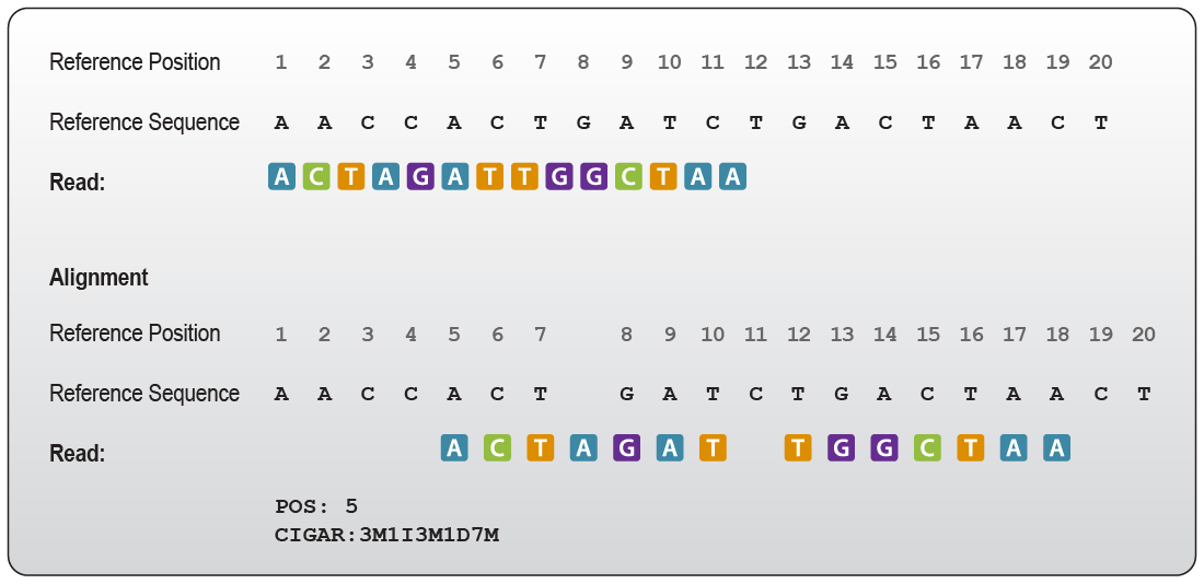
Figure 1 | Example of a CIGAR string for alignments. “POS” defines the position in the reference at which the read alignment starts, in this case, position 5. The CIGAR string states “3M” therefore 3 bases of the read map to the reference. “1I” defines one base that is inserted in the read but does not exist in the reference. This insertion is followed again by 3 bases that map to the alignment indicated by “3M”. Next, one base missing in the read (but present in the reference) is referred to as 1 deleted base “1D”. The last part “7M” defines seven bases that are aligned to the reference. Note that the base on position 14 is a mismatch to the reference, it is counted as mapped as it occupies a position rather than generating an insertion or a gap.
In other types of alignments CIGAR strings also specify clipped bases, mismatches, or longer gaps in case of spliced introns. These alignments per gene or transcript can later be counted to determine their expression. Popular aligners utilized for RNA-Seq are TopHat1, HISAT2 and STAR3. All these aligners can perform gapped alignment. Gapped alignment is essential for RNA-Seq, as splicing of transcripts may lead to large alignment gaps which need to be accounted for (Fig. 2).
The genomic reference contains the complete sequence space of an organism including sequences that are not transcribed (e.g., intergenic sequences without overlaying transcripts) or sequences that are spliced out after transcription (e.g., intron sequences). As RNA-Seq predominantly aims to capture mature transcripts, most of those sequences are also absent from the reads generated in an RNA-Seq experiment. Therefore, two sequences that are next to each other in a read can originate from loci that are much further apart in the genomic reference. Aligners thus need to identify these sequence parts or “seeds” and account for the gap in the alignment (Fig. 2B).
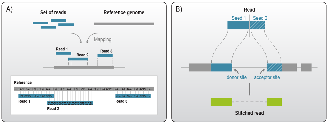
Figure 2 | Read alignment with annotation-based aligners. A) The set of sequencing reads is mapped against a chosen reference genome based on sequence similarity. B) Gapped alignment of RNA-seq reads. When mapping RNA-Seq reads to genomic sequences, aligners need to operate by accounting for gaps. RNA-seq aligners as for instance STAR operate by finding the longest sequence in a read matching the reference genome (seed1). If the read cannot be mapped completely to one continuous sequence, STAR will then try to find the mapping location of the remaining sequence (seed2). The separate seeds are then stitched together to get the alignment position of the read. If this splice junction is not yet known in the reference genome, STAR will also report it as a new junction. Adapted from 3.
Pseudo-aligners
Recently, a special class of aligners, referred to as ‘pseudo-aligners’, have been developed to drastically decrease alignment time. Popular pseudo-aligners like Salmon4, Kalisto5, and Sailfish6 can decrease runtime up to 250-fold, enabling users to quantify their sequenced reads on a simple desktop computer in approximately 10 minutes. Pseudo-aligners utilize sophisticated statistical algorithms to assign a read to a given transcript sequence without mapping the read to the actual genomic location. First, the sequences of all known reference transcripts are broken down into so called k-mers, short subsequences of roughly 30 base pairs. The pseudo-aligner then constructs a network, where these short subsequences serve as nodes. These nodes are then connected by different paths that describe the sequence of a transcript (Fig. 3). The pseudo-aligner then estimates the most likely path (transcript) the sequencing read originates from 5. As a result, pseudo-aligners do usually not output SAM or BAM files, but only tab-delimited quantification tables (although Salmon and Kallisto nowadays can be set to output other file types as well). Therefore, this method reduces the transparency of the quantification process and does not allow the user to look at the read distribution at specific loci. This lack of read distribution may be detrimental when attempting to answer specific research questions. Most pseudo-aligners are also unable to perform read collapsing based on Unique Molecular Identifiers (UMIs) for bulk RNA-Seq data analysis.
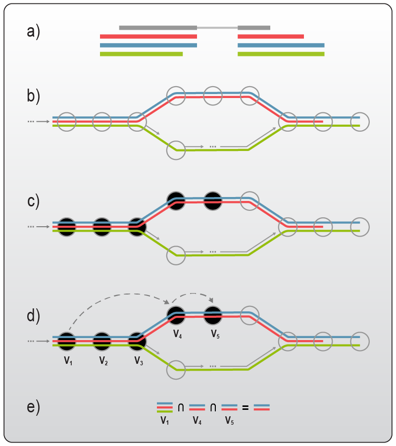
Figure 3 | Read alignment with pseudo-aligners. When using pseudo-aligners such as Kallisto, reference transcripts are broken down into much smaller subsequences (k-mers). These subsequences are then used to construct a network, where each subsequence is a node. In this network, transcripts can be described by a path leading from node to node. Reads that should be pseudo-aligned are then split as well into multiple k-mers, while the algorithm calculates which path (transcript) the deconstructed reads most likely originates from. Figure adapted from 5.
Which Aligner is Best used for your Analysis?
Due to the limitations outlined above, it is recommended to use annotation-based aligners to analyze RNA-Seq data from libraries containing UMIs (e.g., data derived from CORALL library preps) when UMI-based read collapsing is required. Annotation-based aligners, specifically STAR is also recommended when using 3’ mRNA-Seq methods (such as Quantseq), although benefits of using pseudo-aligners were highlighted especially for high-throughput 3’-Seq projects7.
The downside of using annotation-based aligners is that they require a high-quality genome annotation to operate properly. While annotations for model organisms, such as human and mouse genomes, are continuously updated, researchers can be hard pressed to find a decent annotation when working with non-model organisms. In case of 3’-Seq data analysis, a decent 3’ annotation is especially important to maximize the percentage of mapped reads for a meaningful analysis. In this case, pseudo-aligners allow to analyze and quantify expression of transcription units independent of an annotation and thus can offer more information to the researcher.
2. UMI-based Read Collapsing
If UMIs have been utilized during library preparation, UMI-based read collapsing can be performed. In general, this analysis step is optional and UMI-based deduplication can be omitted when working with high input amounts to save computational resources. In any case, the UMI sequence should always be removed before proceeding to the alignment step to ensure unimpaired read mapping (see Chapter 11 for details).
UMI collapsing serves to remove PCR duplicates by reducing them to one read. During PCR, DNA fragments amplify with varying efficiencies. How efficient a fragment is amplified is often based on multiple factors such as length, GC content, secondary structure and the number of PCR cycles that are applied to an NGS library (see Chapter 7 for more details). UMI-based read collapsing can reduce the biases which are introduced during amplification.
While the “duplication rate” assessed by popular sequencing quality control tools such as FastQC can be seen as an indication for the complexity of a data set, UMI deduplication offers a more precise estimation of actual read duplication during the complete sequencing workflow including the PCR step and sequencing itself.
Most bioinformatic tools achieve this by comparing the UMI sequence of reads with the same starting position. Reads with the same UMI are marked as PCR duplicates and collapsed into one single read (see Chapter 8 for a detailed overview of UMIs). The most widely used and recommended software for UMI-based read collapsing is UMI-tools8. Commonly used tools for UMI-based collapsing also offer the possibility to correct for errors within the UMI sequences (Fig. 4).
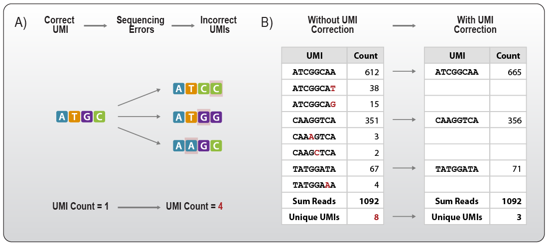
Figure 4 | UMI error correction. A) Sequencing errors introduced into the UMI sequence lead to novel sequences that differ in a limited number of bases, in most cases 1 error is set as default. Counting UMI sequences without error correction would result in a unique UMI count of 4 instead of 1. B) UMI counting with and without error correction. UMIs mapping to the same gene / position are counted to improve quantification of the gene or transcript (see Chapter 8). Counting UMIs that contain sequencing errors without correction overestimates the number of unique UMIs and can thus impact quantification. During the correction step, the UMI with the highest number of assigned reads is assumed as correct or parent sequence. UMIs that differ in 1 base have a Hamming Distance of 1 and are likely derived from the parent UMI (see Chapter 9 for more information on sequence distances). Thus, UMI error correction will group these UMI sequences reducing the count of unique UMIs for the respective gene / position.
UMI-tools does this by building a nearest neighbor network of UMI sequences for all reads at a specific mapping location. UMIs that can be derived from each other with a substitution of one base (or a higher user defined threshold) will be connected and grouped together in one network. This network is then used to identify potential sequencing errors in the UMI based on the network connectivity and collapse the corresponding reads. Depending on the research question, error correction during UMI collapsing can improve the accuracy of the data.
The percentage of reads that are collapsed based on their UMI during this step largely depends on the experimental setup:
- Input RNA amount: processing of limited RNA inputs often requires more PCR cycles for amplification and generates libraries with lower complexity. As a consequence, a large number of reads can be collapsed during this step, especially when sequencing at saturated depth.
- Complexity of the sample: higher collapsing rates are seen for samples which are low in complexity due to a lower diversity.
- Sequencing depth: at saturated sequencing depth, a larger fraction of reads is expected to be removed by collapsing. At which per-sample-sequencing-depth saturation is reached depends on the complexity of the sample itself, the input amount, and the efficiency of the library preparation. For samples with low complexity, at low input amounts or for library preps with low efficiency, saturation is reached earlier at lower depth per sample.
For example, sample types with a lower complexity or limited input material are expected to show higher fractions of collapsed reads, especially when sequencing has reached saturation, i.e., when higher sequencing depth is applied than needed (over-sequencing). As over-sequencing provides little gain in relation to the additional cost, UMIs are very useful to determine the “sweet-spot” of per-sample-sequencing-depth, especially for large scale projects. UMI collapsing rates at different sequencing depths (e.g., using sub-sampling of reads) can thus be used to determine how many reads per sample are optimal for the research question under investigation. This allows to save sequencing costs by avoiding over-sequencing and by multiplexing more samples per run at optimal depth.
3. Quantification
During quantification, reads mapping to specific genes or transcripts are counted to provide a direct readout of gene expression. Many popular quantification tools are available, such as featureCounts9, RSEM 10 and Salmon4. Lexogen has also developed a unique proprietary quantifier, Mix² 11, which quickly and accurately estimates transcript concentrations.
Most bioinformatic tools for differential gene expression, a popular tertiary analysis, use raw counts as input. While raw counts are the output of all quantifiers, many also provide differently normalized expression values. Hence, quantification tools have different specializations. Therefore, it is important to consider the research question at hand and library type when selecting a quantifier. The inputs for most quantifiers are usually a SAM or BAM file, which contains the aligned reads and a genome annotation. The quantifier then determines the number of reads overlapping with annotated transcripts or genes. FeatureCounts, one of the most minimalistic quantifiers available, returns a count table for each gene or transcript making it an especially useful tool for 3’ RNA-Seq methods where reads are localized to the 3’ ends of transcripts. Thus, 3’ RNA-Seq data sets do not require fitting of sequencing reads over the complete transcript length and can also forego transcript quantification estimation.
For example, due to QuantSeq’s straightforward one-read-per-transcript chemistry and the resulting simplicity of analysis, featureCounts is recommended for quantifying QuantSeq data.
In contrast, limitations apply when counting is used on whole transcriptome (WTS) data sets. As longer transcripts naturally receive more counts than shorter ones, counting introduces a length bias leading to a relative inaccuracy between different transcript length classes in one sample. Therefore, these data sets are commonly analyzed with tools allowing for transcript concentration estimation, such as RSEM, Salmon or Lexogen’s Mix². Next to raw counts and length all three of these algorithms return normalized expression values such as FPKM (Fragments per kilobase of exon per million fragments mapped) or TPM (Transcripts per million). This allows the researcher to compare expression values of genes of varying lengths within one sample.
Data analysis for Lexogen libraries differs slightly from the commonly used settings for analysis of data generated from other vendor’s library preps. Most of the library preps developed by Lexogen generate reads in forward orientation, i.e., Read 1 reflects the sequence of the RNA transcript (Fig. 5).
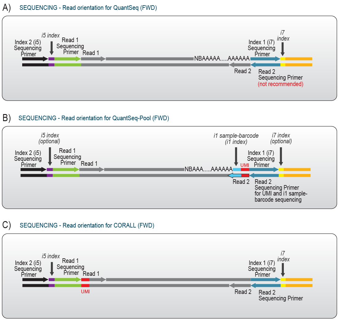
Figure 5| Read orientation for A) QuantSeq, B) QuantSeq-Pool, and C) CORALL libraries. For all libraries, Read 1 is in forward orientation and thus corresponds to the transcript sequence. While the UMI and inline index for QuantSeq-Pool libraries is located at the beginning of Read 2, the UMI sequence for CORALL libraries is read out at the beginning of Read 1. Optionally, a UMI can also be introduced in classical QuantSeq libraries. In this case, the UMI is also located at the beginning of Read 1 (not shown).
In contrast, many conventional library preps generate reads in reverse orientation, i.e., Read 1 reflects the sequence of the cDNA, the reverse complement of the RNA transcript.
Researcher therefore need to take care when using freely available tools for data analysis as standard settings may reflect reverse read orientation. Performing data analysis steps with incorrect read orientation is known to produce false results, for example for genome wide coverage analysis. Gene body coverage plots are calculated from the coverage distribution across a set of abundant genes along their normalized length. As they are often used as a quality parameter, a false read orientation setting will give the impression of a poor-quality data set. Further, gene and transcript quantification will be affected if the read orientation is set incorrectly.
UMIs can also often be difficult for researchers to process. In general, the position of UMIs is variable and depends on the respective library prep itself. Most UMIs are positioned at the beginning of Read 2 and require (partial) paired-end read mode during sequencing, as for example in QuantSeq-Pool libraries (Fig. 5). In contrast, for QuantSeq FWD and CORALL, the UMI is located at the beginning of Read 1 and is thus naturally a part of Read 1 (Fig. 5). As such, the UMI needs to be extracted prior to the alignment step to avoid interference during mapping as described in Chapter 11.
To facilitate data analysis for our users, Lexogen offers various plug-and-play data analysis solutions at partner platforms as well as a set of pipelines and tools on Github. For more information on data analysis solutions, visit our online FAQ page.
The expression information generated during the quantification step is the basis for more advanced tertiary analysis. In our final Chapter on Data Analysis, we will explore the most common applications for tertiary analysis and add further insights on quality control steps that will help you to make the most of your RNA-Seq data.
Written by W. Falko Hofmann, PhD and Dr. Yvonne Goepel
Are you ready to become an RNA Expert?
Sign up and gain access to helpful checklists in PDF format that can assist you in your experiments. In addition, you’ll have the opportunity to download the RNA LEXICON E-BOOK in PDF format as well.
Literature:
1 Kim, D., Pertea, G., Trapnell, C. et al. (2013) TopHat2: accurate alignment of transcriptomes in the presence of insertions, deletions and gene fusions. Genome Biol. 14: R36. doi:10.1186/gb-2013-14-4-r36
2 Kim, D., Langmead, B. and Salzberg, S. (2015) HISAT: a fast spliced aligner with low memory requirements. Nat. Methods 12: 357–360. doi:10.1038/nmeth.3317
3 Dobin, A., Davis, C. A., Schlesinger, F., et al. (2013) STAR: ultrafast universal RNA-seq aligner. Bioinformatics 29: 15–21. doi:10.1093/bioinformatics/bts635
4 Patro, R., Duggal, G., Love, M. et al. (2017) Salmon provides fast and bias-aware quantification of transcript expression. Nat. Methods 14: 417–419. doi:10.1038/nmeth.4197
5 Bray, N., Pimentel, H., Melsted, P. et al. (2016) Near-optimal probabilistic RNA-seq quantification. Nat. Biotechnol. 34:525–527. doi:10.1038/nbt.3519
6 Patro, R., Mount, S. & Kingsford, C. (2014) Sailfish enables alignment-free isoform quantification from RNA-seq reads using lightweight algorithms. Nat. Biotechnol. 32:462–464. doi:10.1038/nbt.2862
7 Corley, S.M., Troy, N.M., Bosco, A. et al. (2019) QuantSeq. 3′ Sequencing combined with Salmon provides a fast, reliable approach for high throughput RNA expression analysis. Sci. Rep. 9: 18895. doi:10.1038/s41598-019-55434-x
8 Smith, T., Heger, A., Sudbery, I. (2017) UMI-tools: modeling sequencing errors in Unique Molecular Identifiers to improve quantification accuracy. Genome Res. 27:491-499. doi:10.1101/gr.209601.116
9 Liao Y, Smyth GK, Shi W. (2014) featureCounts: an efficient general purpose program for assigning sequence reads to genomic features. Bioinformatics. 30:923-30. doi:10.1093/bioinformatics/btt656
10 Li, B., Dewey, C.N. (2011) RSEM: accurate transcript quantification from RNA-Seq data with or without a reference genome. BMC Bioinformatics 12: 323. doi:10.1186/1471-2105-12-323
11 Tuerk, A., Wiktorin, G., and Güler, S. (2017) Mixture models reveal multiple positional bias types in RNA-Seq data and lead to accurate transcript concentration estimates. PLoS Comput. Biol. 13: e1005515. doi:10.1371/journal.pcbi.1005515