In our previous Chapter 8, we introduced Unique Molecular Identifiers (UMIs) as tags to mark each individual molecule within a sample. In this chapter of the RNA LEXICON, we will focus on a different kind of tag, namely indices. Indices specifically mark each sample in a sequencing experiment and allow simultaneous analysis of many samples in one sequencing run.

1. Sample Multiplexing
High-throughput sequencers produce billions of reads in a single run, heavily outweighing the read depth requirement for single samples which typically lies between 1 M and 100 M reads. Therefore, it is desirable to combine (or “multiplex”) libraries from various samples or experiments in one sequencing run. For multiplex sequencing, defined index sequences are added to each library during the Next-Generation Sequencing (NGS) library generation workflow. Each individual molecule generated from an initial RNA sample will have the same index. In contrast, molecules generated from other samples will be tagged with different indices. After sequencing, each read can be identified and associated to the sample it derived from based on the index sequence with which it was tagged. The index tags are typically short defined sequences between 6 – 12 nucleotides. These tags are then read out during the sequencing run.
There are two main strategies for indexing which are commonly used: inline indexing (or sample-barcoding) and multiplex indexing which we will explore in the following sections.
2. Inline Indexing / Sample-barcoding
Inline indices or sample-barcodes are located between the sequencing adapter and the insert (Fig. 1 shows an inline index located at the beginning of Read 2). Due to their positioning, inline indices are part of the insert read, and must be read out either in Sequencing Read 1 or Read 2. Consequently, the read length available for sequencing the actual insert will be reduced by the length of the inline index.
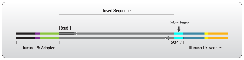
Figure 1 | Inline indices are commonly located at the beginning of Read 2. Read out of inline indices occurs during insert reads and is independent from the multiplex indices located within the Illumina adapter sequences. It is also possible that inline indices are located at the beginning of Read 1 (not shown).
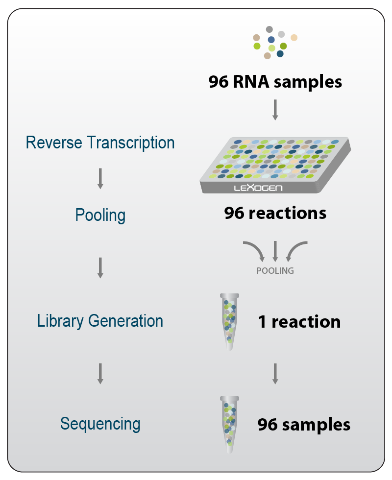
Figure 2 | Inline indexing (sample-barcoding) allows early pooling thereby streamlining the complete workflow. This enables significant savings for consumable and effectively shortens the overall hands-on time to complete library preparation. Additionally, throughput can be upscaled to tens of thousands of samples.
Inline indices or sample-barcodes are commonly introduced in the first step. The index sequence is added to the reverse transcription primer and is therefore mostly located at the beginning of Read 2. Thus, libraries containing inline indices commonly require paired-end sequencing with at least a partial read-out of Read 2.
These indices are commonly used in applications requiring ultra-high throughput. As inline indices are added to the molecules directly in the first step, they allow combination of all indexed samples for subsequent reaction steps. As a result, hundreds of samples can be handled in parallel and multiplexing capacity can be increased to process thousands of samples in one experiment, as exemplified by the QuantSeq-Pool workflow (Fig. 2). Therefore, inline indexing strategies are often pursued for high-throughput screening experiments and for massive single-cell sequencing studies.
Using library preps containing inline indices is not only a convenient way to increase sample throughput, but also saves a lot of consumables as the samples are pooled early and processed in batch. This also effectively shortens hands-on time and can decrease technical variance. For an introduction to sample-barcoded 3’ mRNA-Seq check out our RNA EXPERTise video on QuantSeq-Pool.
3. Multiplex Indexing
Continuous improvements in the NGS technology are aimed towards increasing sequencing speed and data output for massive sample throughput. A key to utilizing this increased capacity is multiplex indexing. Just like inline indexing, multiplex indexing allows multiple libraries to be sequenced simultaneously. In contrast to inline indices, multiplex indices are located within the common sequencing adapters and require designated Index Reads to be assessed (Fig. 3). Thus, multiplex indices do not have an impact on the insert read length.
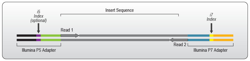
Figure 3 | Multiplex indices are located within the Illumina Adapters. Dedicated Index Sequence Reads are required to assess multiplex indices. Different indexing strategies can be applied: single indexing only uses the i7 index (Index 1), while dual indexing uses both, the i7 (Index 1) and the i5 index (Index 2).
As multiplex indices are part of the common sequencing adapters, they are introduced at a later step in library generation, either during adapter ligation or during the final PCR amplification step.
Multiplex indexing comes in different flavors: single indexing where only Index 1 (the i7 index) is used, and dual indexing that uses both, Index 1 and Index 2 (the i5 index) either in combinatorial mode or as unique index sequence pairs.
4. Multiplex Dual Indexing – Practical Implications
Dual indices can be applied in two different ways – either in a combinatorial or in a non-redundant (= unique) manner. Combinatorial dual indexing uses each individual i5 and i7 index multiple times whereby each combination of these indices is only used once in the experiment (Fig. 4).
This allows a tremendous increase in multiplexing capacity and concomitantly reduces the overall per-sample cost. However, as the barcodes are shared between multiple samples, it is not always possible to unambiguously identify the corresponding sample in case of index sequence errors.
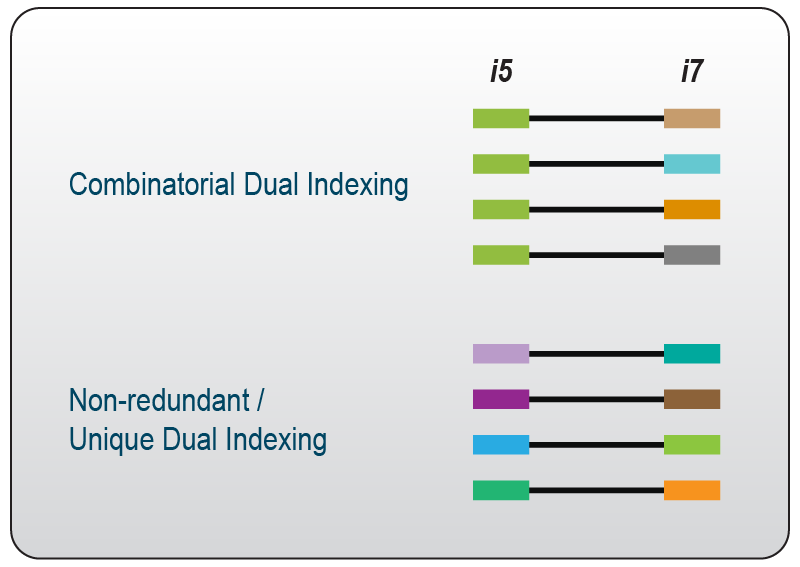
Figure 4 | When using combinatorial dual indexing, every i5 and i7 is used multiple times; therefore, the combinations are unique, the individual indices are not. In contrast, when using unique dual indexing, each i5 and i7 index is used only once; every combination and every index is therefore unique.
When following a unique dual indexing strategy on the other hand, each individual i5 and i7 index is used only once in the experiment (Fig. 4). As a result, index crosstalk can be dramatically reduced, and index mis-assignment can be prevented3.
In case of errors, the second index of the pair can be used as a reference point to pinpoint the identity of the original index pair. This ultimately has the potential to salvage a large fraction of otherwise unassigned reads by reverting the erroneous sequence back to the original sequence in a process termed “index error correction”. In typical sequencing experiments, ~10 % of the reads cannot be assigned and would therefore be discarded when error correction is not applied.
Unique Dual Indices (UDIs) are recommended for best practice and for the highest possible accuracy for demultiplexing / index assignment.
Advantages of Unique Dual Indexing
- UDIs increase the accuracy of sample identification by using two unique identifiers.
- UDIs enable identification of index errors and index-sample-swaps or index hopping. This is not possible when single indexing is used. As the i5 index is lacking, there is no second reference point to assess which sample the read originated from when the i7 index is changed to an ambiguous sequence, i.e. it could have originated from another sample.
- Well-designed UDIs are the basis for index error correction. Index error correction can rescue unassigned reads that would otherwise be discarded. As a practical example, the ~10 % of discarded reads from a NovaSeq (S4 FlowCell) can account for up to two full NextSeq500 runs, or up to 800 M reads, which can be saved when using UDIs and error correction.
- Ultimately, UDIs reduce per-sample costs and maximize sequencing output.
5. Index Sequence Design – From Distances to Indices
Index sequence design is extremely important for the improvement in accuracy that unique dual indexing can offer, and it determines the error correction capacity of the index set. In this section, we will dive into design features and explain what makes an index set truly advanced. One obvious requirement for index sequence design is to provide the necessary color- and nucleotide-balance to ensure a high enough complexity for a smooth sequencing process and signal detection. A major factor that determines the quality of any given index set is the inter-index distance (also referred to as inter-barcode distance).
The inter-index distance is a measure of dissimilarity between sequences in a given set. The distance is defined as the number of edit events that are required to transform any one sequence into any other sequence of the same set. The higher the inter-index distance, the more edit events are needed for this transformation. Or in other words: the larger the inter-index or edit distance, the more unlikely it is to create false-positive barcode matches, and the easier it becomes to detect and correct erroneous index sequences.
“Edit events” summarizes all types of errors that can modify the nucleotide composition of a sequence, i.e., nucleotide substitutions, where one base is exchanged for another at the same position or any changes that alter the positioning of nucleotides in the sequence context, such as insertions, where a base is added and deletions where a base is removed (Fig. 5).
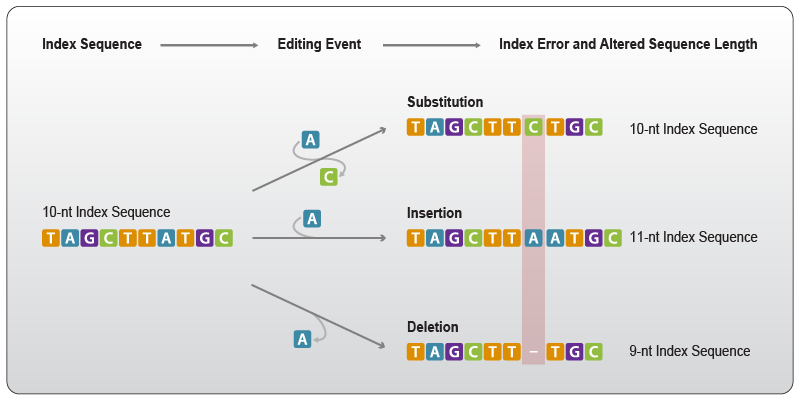
Figure 5 | Edit events change defined into unknown sequences. Substitution: a base in the sequence is replaced by another base, e.g., an adenosine is substituted by a cytosine. Insertion: a base, e.g., adenosine, is added at any given position; all following bases are shifted by one position generating a longer sequence. Deletion: a base, e.g., adenosine, is removed at any given position; all following bases are shifted by one position generating a shorter sequence.
Key Principles for Illumina-compatible Index Sequence Design
- Color- and nucleotide balance should be considered in the design to ensure efficient sequencing and signal detection on the machine. Illumina machines using 2-color chemistries (i.e., only two fluorophores are used to distinguish the four different nucleotides) may require a higher nucleotide diversity than machines applying 4-color chemistry and a different fluorophore for each nucleotide.
- Index Sequence length: longer index sequences have a higher inter-index distance than shorter index sequences. Longer sequences possess a more complex sequence space, i.e., more possible nucleotide combinations. Due to the higher number of overall possible sequences the ones with the largest index-distances can be chosen.
- The inter-index distance chosen for the design has implications on the types of errors that can be detected and corrected. The following index distances are commonly used: Hamming distance, Levenshtein distance, and Sequence-Levenshtein distance, as well as modifications thereof. To learn more about these distance types and their implications for index design, see below.
The Hamming distance was introduced by Richard W. Hamming in the 1950s and is a measure for dissimilarity between two strings of characters that are equal in length. In terms of index sequences the Hamming distance can be used to describe the number of positions in which the bases of two index sequences differ. It measures the minimum number of substitutions required to change one sequence into the other.
While the Hamming distance is used for binary strings, it can also be explained as using a codeword scheme. For example, it can be applied to words of equal length. To transform the name “Addison” into “Allison”, only two letters need to be exchanged. Therefore, the Hamming distance between Addison and Allison is 2.
As the Hamming distance requires both sequences to be of equal length, deletions and insertions cannot be assessed (see Fig. 5). One downside of not being able to take insertions and deletions into account is that a large Hamming distance does necessarily reflect a large edit distance (Fig. 6).
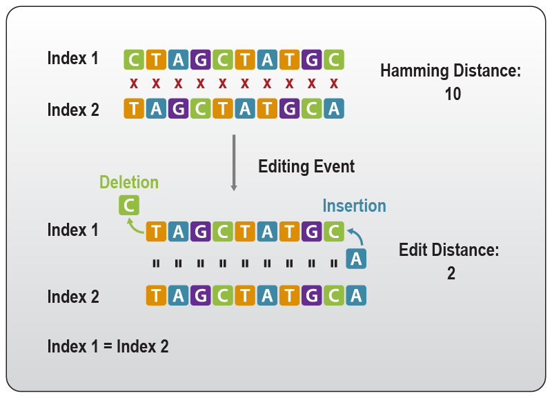
Figure 6 | Insertions and deletions reduce the usability of Hamming-based Index sequences. Two indices that are different from one another by 10 substitutions (Hamming distance = 10) can have an edit distance of two, i.e., that a total of two insertions or deletions can turn Index 1 into Index 2 leading to sample misassignment. Adapted from4.
Therefore, the Hamming distance may not be the most appropriate design parameter to ensure sophisticated index sequence design. Rather, modifications of the Levenshtein distance are used to account for editing events other than substitutions.
The Levenshtein distance is another string metric to describe the difference between two sequences. It was introduced by Vladimir Levenshtein in the 1960s. The Levenshtein distance between two sequences is defined as the minimum number of single-character edits required to change one sequence into the other. In contrast to the Hamming distance, the Levenshtein distance can also assess substitutions and deletions and allows to compare sequences of variable lengths (Fig. 7).
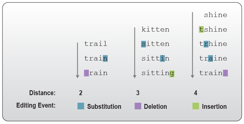
Figure 7 | Levenshtein distance as exemplified by the transition from one word into another. The transition from “trail” to “rain” requires at least 2 edits and thus has a distance of 2. The Levenshtein distance between “kitten” and “sitting” is 3, and between “shine” and “train” it is 4 as at least 4 editing events are required to change one into the other. Editing events are defined as either insertion, deletion, or replacement of a character (substitution).
The Levenshtein distance is more flexible than the Hamming distance and can cover all editing events that can occur at index positions during a sequence workflow. The NGS-specific problem that arises for the classic Levenshtein distance is that during a sequencing experiment, the read-out is fixed. For example, the index read will always be 10 imaging cycles, i.e., 10 nucleotides will be read out even when the index length is changed to 9 nucleotides by deletion or 11 nucleotides by insertion. This means that “non-index nucleotides” will be moved into the sequencing frame in the course of deletions and “index-nucleotides” will be moved out of the sequencing frame upon nucleotide insertions.
As a consequence, the Levenshtein distance as originally conceived is also not optimal for index sequence design.
While the length of the index is known per design, the length of the actual observed index in a sequencing experiment can be altered and is thus an unknown variable.
In case of nucleotide deletions, the nucleotides located downstream of the sequencing frame are moved into the index space. If the index length is increased by nucleotide insertions, bases belonging to the original index sequence are moved out of the index space and now precede the nucleotides of the adapter or insert (Fig. 8). These bases will not be seen in the data as the index reads are usually not increased beyond the original index boundaries.
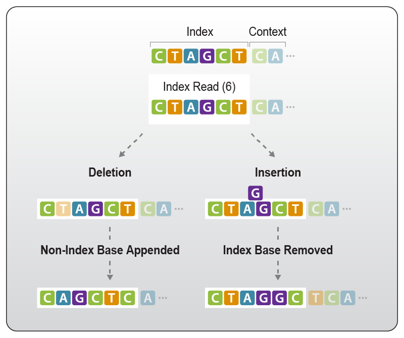
Figure 8 | Impact of deletions and insertions on the index read-out. Upon deletions within the index sequence, non-index bases succeeding the index nucleotides enter the frame of the index read. Insertions within the index sequence leads to index-associated bases to move out of the index read frame. They now precede the downstream sequence, i.e., either the adapter sequence when multiplex indices are used or the insert sequence when inline indices are used.
The Sequence-Levenshtein distance is a variation of the original Levenshtein distance described above, it is adapted to account for the sequence context in a continuous flow. It can account for changes caused by appended non-index nucleotides and the resulting shorter distance between the read-out index sequence. Thereby the actual length of the erroneous index can be correctly identified as well as appended nucleotides5. Nucleotides that move in and out of the index space can generate sequences with shorter distances to other indices in the set as compared to the original index sequence they are derived from. A large inter-barcode distance based on the Sequence-Levenshtein distance, therefore, does not necessarily guarantee accurate error correction.
Further advances in this field improve index sequence design by accounting for the probability of deletions, substitutions, and insertions in sequencing experiments and focusing on the shifts that can be caused at the 3’ end of the index sequence6.
Here at Lexogen, we strive to improve every step of the sequencing process. Therefore, Lexogen has designed and produced the most sophisticated Unique Dual Index (UDI) Set on the market to date. The result is a versatile, scalable, and nested UDI Set with maximized inter-index distance for all sample sizes. Ultimately, these UDIs enable superior error-correction and allow for tremendous cost savings through maximized sequencing output by rescuing the majority of unassigned reads.
6. The Best of Both Worlds – Combining Indexing Strategies
Combining inline and multiplex indexing allows to take sample multiplexing even further: experiments can be easily scaled up to tens of thousands of samples for ultra-high throughput applications, such as massive screening projects. The combination of inline indices and UDIs in a triple index system enables highly confident sample assignment for more than 36,000 individual samples, e.g., 96 sample barcodes combined with 384 UDIs, 96 x 384 = 36,864 (Fig. 9).
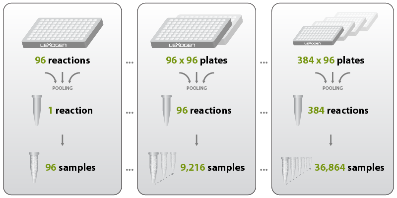
Figure 9 | Highly scalable throughput and confident sample assignment by combining inline indexing (sample-barcoding) with unique dual multiplex indices. For example, combining 96 inline indices with 96 or 384 UDIs allows multiplexing of 9,216 or 36,864 samples and thus provides a cost-efficient solution for large scale screening approaches.
7. Some Actionable Advice – The Connection between Flow Cell Chemistries, Instruments, and Indexing
While Unique Dual Indexing is the gold standard for RNA-Seq, the characteristics of sequencing instruments themselves can impact the run performance in a way that can influence the choice of indexing strategy. By far, the most common sequencing instruments used are those made by Illumina, whose sequencer portfolio utilizes two separate types of flow cells: patterned, and non-patterned (also known as random flow cells).
Non-patterned flow cells have a uniform surface on which cluster generation occurs randomly across the flow cell. Provided the user loads the flow cell with the appropriate concentration, cluster generation will generally succeed without issue (Fig. 10, left). Now, advancements have resulted in the adoption of a patterned flow cell, where the surface of the flow cell is occupied by billions of nano-wells in which the cluster generation is occurring within a known, defined physical space (Fig. 10, right). There are a number of advantages to the patterned flow cell. The cluster generation is more tolerant of a wide range of loading concentrations, since the nano-wells reduce the chance of over-loading the flow cell. Also, because the nano-well locations are known, there is no need to map the cluster sites, saving time during sequencing.
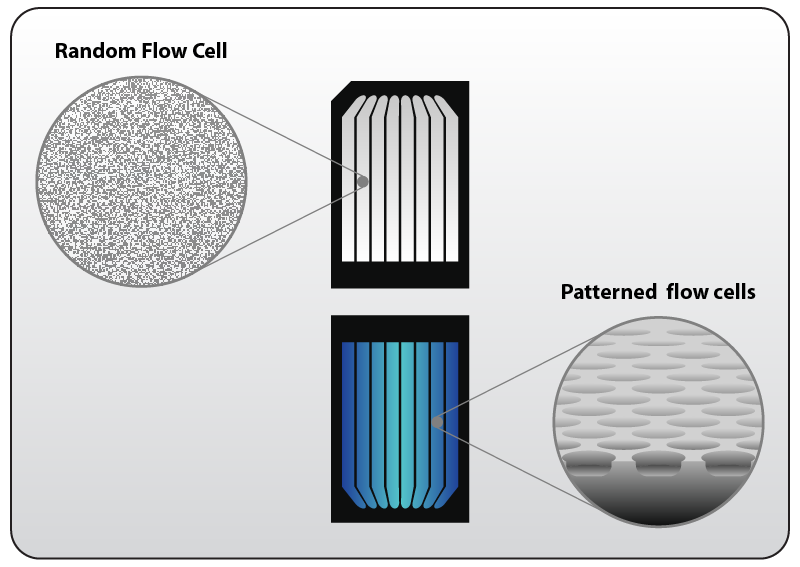
Figure 10 | Random and Patterned flow cell for Illumina Sequencers. Left: Clustering on random / non-patterned flow cells occurs randomly by library molecules binding to flow cell oligos attached to the surface. Clustering is influenced mainly be the loading concentration of libraries. Right: Patterned flow cells are characterized by regularly spaced nano-wells that contain the flow cell oligos. Cluster generation occurs only within the nano-wells making the flow cell less sensitive to overclustering while increasing cluster density and concomitantly data output. Find more information on www.illumina.com.
That being said, there is one major drawback to the patterned flow cell, which is the increase in index hopping events2. The patterned flow cell uses a different type of sequencing chemistry, dubbed Exclusion Amplification, or ExAmp chemistry. This replaces the bridge amplification method previously used for cluster generation on non-patterned flow cells. In ExAmp chemistry, all of the reagents needed for cluster generation are mixed before the cluster generation occurs, which is the likely cause of index swapping as there are free index primers in the mix ahead of cluster generation. Whereas in the traditional bridge amplification chemistry, these free index primers are removed in a washing step after hybridization of DNA to the flow cell. It is estimated that up to 6 % of reads on patterned flow cells can be affected by index switching, compared to less than 1 % on non-patterned flow cells7.
The benefits of the patterned flow cell are significant, and this is shown in the sweeping adoption of them across the Illumina sequencer family. The ease of loading and shortened sequencing time are major benefits as the amount of multiplexing increases continually. Therefore, it is imperative to use the available tools to mitigate the unavoidable increase in index hopping events introduced by the patterened flow cell technology. For best practice, it is strongly recommended to use the unique dual indexing strategies outlined in this chapter, particularly those with the capacity for error correction, which can rescue a truly substantial quantity of reads.
Literature:
1 Kircher, M., Sawyer, S., & Meyer, M. (2012). Double indexing overcomes inaccuracies in multiplex sequencing on the Illumina platform. Nucleic acids research, 40:e3, doi: 10.1093/nar/gkr771
2 Illumina White paper. Effects of Index Misassignment on Multiplexing and Downstream Analysis.
3 MacConaill, L.E., Burns, R.T., Nag, A. et al. Unique, dual-indexed sequencing adapters with UMIs effectively eliminate index cross-talk and significantly improve sensitivity of massively parallel sequencing. BMC Genomics 19, 30 (2018), doi: 10.1186/s12864-017-4428-5
4 Faircloth, B.C., and Glenn, T.C. (2012) Not All Sequence Tags Are Created Equal: Designing and Validating Sequence Identification Tags Robust to Indels. PLoS ONE 7(8): e42543, doi: 10.1371/journal.pone.0042543
5 Buschmann, T., and Bystrykh, L.V. (2013) Levenshtein error-correcting barcodes for multiplexed DNA sequencing. BMC Bioinformatics 14, 272, doi: 10.1186/1471-2105-14-272
6 Hawkins, J. A., Jones, S.K., Finkelstein, I.J., and Press, W. H. (2018) Indel-correcting DNA barcodes for high-throughput sequencing. Proceedings of the National Academy of Sciences, 115:E6217-E6226, doi: 10.1073/pnas.1802640115
7 Costello, M., Fleharty, M., Abreu, J. et al. Characterization and remediation of sample index swaps by non-redundant dual indexing on massively parallel sequencing platforms. BMC Genomics 19, 332 (2018), doi: 10.1186/s12864-018-4703-0
Written by Dr. Yvonne Goepel
Are you ready to become an RNA Expert?
Sign up and gain access to helpful checklists in PDF format that can assist you in your experiments. In addition, you’ll have the opportunity to download the RNA LEXICON E-BOOK in PDF format as well.